Theory regarding the uncertainty

Model parameters are computed from a sample (the data from our AWS network in our case) to estimate the parameters of the whole population (our grid). Models actually generalize what is learnt on a sample on the whole population. So the question arises whether we can use this generalization with enough confidence (can we extrapolate these parameters to the whole population) ?

To answer this question, 2 tools are commonly used :

• the standard error
  
• the confidence interval

The standard error is what quantifies the uncertainty while the 95% confidence intervals represent quantiles between which are found 95 % of the samples means after removing the 2.5 % of both the bigger and smaller values. A good explanation of its meaning can be found here and here

In the paper Spatial uncertainty analysis: propagation of interpolation errors in spatially distributed models, the uncertainty is depicted as the standard error of the predictions.

We can also cite the Spatial interpolation of air pollution measurements using CORINE land cover data paper :

When solving the Ordinary Kriging equations, a value for the error variance can be obtained at the same time (Isaaks et al. 1989). This error variance is a measure for the uncertainty of the interpolation result

As a reminder, here are some definitions useful to understand what the standard error exactly is:

• The standard error (SE) of a statistic (usually an estimate of a parameter) is the standard deviation of its sampling distribution.

• The standard deviation is the positive square root of the variance. The standard deviation is expressed in the same units as the mean is, whereas the variance is expressed in squared units.

• The variance is the average squared dispersion around the mean. Variance is a measurement of the spread between numbers in a data set. The variance measures how far each number in the set is from the mean. Variance is calculated by taking the differences between each number in the set and the mean, squaring the differences (to make them positive) and dividing the sum of the squares by the number of values in the set.

How to extract the uncertainties of predictions using R ?

Let’s find an example on the web. Tomislav Hengl, an expert in the field of geostatistics has published a nice tutorial about how to vizualize spatial uncertainty. In his tutorial, he uses the se output of the krige function as the uncertainty indicator. (krige doc, is a simple wrapper method around gstat and predict). The code here below comes from his tutorial

library(rgdal)
library(maptools)
library(gstat)

# using the Meuse dataset
data(meuse)
coordinates(meuse) <- ~x+y
data(meuse.grid)
gridded(meuse.grid) <- ~x+y
fullgrid(meuse.grid) <- TRUE

# universal kriging:
k.m <- fit.variogram(variogram(log(zinc)~sqrt(dist), meuse), vgm(1, "Sph", 300, 1))
vismaps <- krige(log(zinc)~sqrt(dist), meuse, meuse.grid, model=k.m)
names(vismaps) <- c("z","e")

# Plot the predictions and the standard error :
z.plot <- spplot(vismaps["z"], col.regions=bpy.colors(), scales=list(draw=TRUE), sp.layout=list("sp.points", pch="+", col="black", meuse))
e.plot <- spplot(vismaps["e"], col.regions=bpy.colors(), scales=list(draw=TRUE))

print(z.plot, split=c(1,1,2,1), more=TRUE)
print(e.plot, split=c(2,1,2,1), more=FALSE)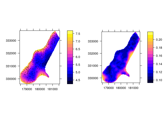

Meuse data Kriging + uncertainty

Nice we have what we need ! Easy ! But how are SE computed for the predictions ? We could have a look at the source code of the krige function. But let’s build it manually with a simple example for the sake of comprehesion. Doing so, requires some matrix algebra (variance + covariance matrix). A detailed explanation of the next code block is available in this course

# example from @frdvwn

# creating a sample
set.seed(123)
n <- 100
n.lev <- 10
alpha <- 10
beta <- 1.3
sigma <- 4

x <- rep(1:n.lev,each=n/n.lev)
y <- alpha - beta*x + rnorm(n,0,sigma)

# vizualizing the dataset
plot(x,y)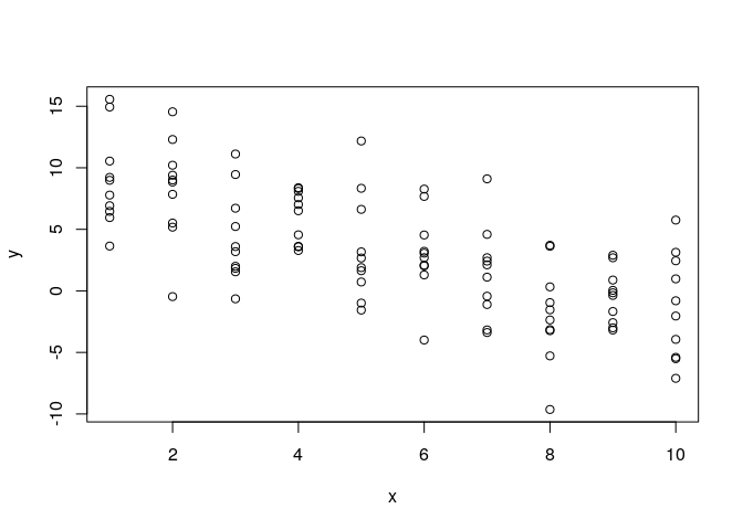

Meuse plot

# modelizing
mod <- lm(y~x)

# creating the points on which we want to predict values using the model equation
X <- cbind(1,seq(0,10,0.01))
beta <- coef(mod)

# Predicting manually using matrix algebra
y.hat <- X %*% beta
V <- as.matrix(vcov(mod))
y.hat.se <- sqrt(diag(X %*% V %*% t(X)))

# Predicting using predict function
auto.y.hat.se <- predict(object = mod, newdata = data.frame(x=X[,2]), se.fit=TRUE)$se.fit

# Vizualizing the SE
plot(y~x)
lines(y.hat ~ X[,2],col="red")
lines(y.hat + y.hat.se ~ X[,2],col="red",lty=2)
lines(y.hat - y.hat.se ~ X[,2],col="red",lty=2)
lines(y.hat + auto.y.hat.se ~ X[,2],col="green",lty=2)
lines(y.hat - auto.y.hat.se ~ X[,2],col="green",lty=2)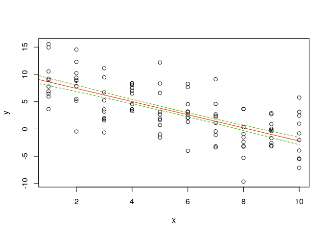

Meuse plot with SE

# same values ? 
print(head(auto.y.hat.se))

    ##         1         2         3         4         5         6 
    ## 0.7905189 0.7893898 0.7882612 0.7871330 0.7860052 0.7848779

print(head(y.hat.se))

    ##         1         2         3         4         5         6 
    ## 0.7905189 0.7893898 0.7882612 0.7871330 0.7860052 0.7848779

Ok we have succeeded to manually compute the Standard errors of the predictions !